
Ultrasound Knobology Guide
Published
Why Knobology Matters More Than Presets
Every modern ultrasound machine ships with a generous library of presets. Liver. Carotid. OB second trimester. Cardiac adult. They are useful starting points and they are also a trap. Presets are vendor assumptions about an average patient performing an average study under average conditions. Your patient is not the average patient, your room lighting is not the manufacturer's lab, and the question your interpreting physician needs answered is rarely the average one. Consistently diagnostic images — and a solid footing for the SPI and clinical specialty exams — come from understanding what each control is actually doing to the underlying physics, and from confidently moving off-preset to optimize for the patient and pathology in front of you.
This guide is a vendor-neutral, physics-first walkthrough of every operator-controlled setting on a modern ultrasound system. For each control we cover what it does, the physics behind it, when to increase, when to decrease, the trade-off you accept, and how that control tends to be tested on the SPI exam. It is written for two audiences at the same time. New sonographers and students preparing for boards will use it as a structured map of the front panel. Working sonographers adding a registration or refreshing for CME will find it a useful physics-anchored refresher tied directly to the exam content outline. If you want a deeper dive into the SPI exam itself, our companion post on the complete ARDMS SPI exam guide pairs naturally with this one.
A Quick Mental Model: The Three Image Quality Currencies
Before we touch a single knob, it helps to name the three currencies you are constantly trading among. Almost every adjustment on the machine spends one to buy more of another.
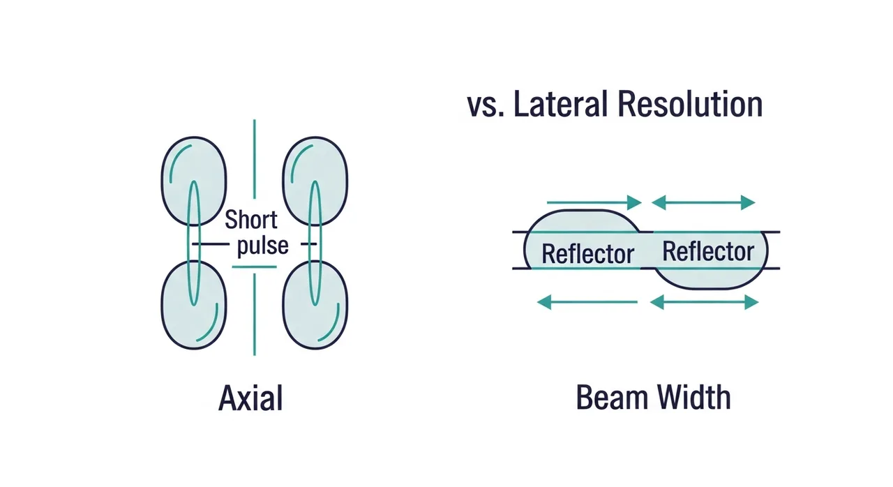
Spatial resolution is the ability to distinguish two structures that are physically close together. It has two flavors: axial resolution along the beam, governed by spatial pulse length and therefore by frequency and bandwidth, and lateral resolution across the beam, governed by beam width at the depth of interest.
Temporal resolution is frame rate — how many complete images per second the machine produces. High temporal resolution captures rapid motion (a fetal heart, a moving valve, a turbulent jet) without blur.
Sensitivity and penetration is the ability to recover usable echoes from deep structures and from low-amplitude reflectors. It is bought primarily with lower frequency, more power, more averaging, and longer dwell time.
Almost every knob on the panel moves you along one of these axes at the cost of another. Once you internalize that, knobology stops being a list to memorize and starts being a set of intentional trades.
B-Mode Controls
Frequency and Transducer Selection
What it does: Selects the center operating frequency of the transducer, either by switching probes or by selecting a frequency band on a multi-frequency probe.
Physics: Axial resolution is roughly half the spatial pulse length, and pulse length shrinks as frequency rises. Higher frequencies therefore resolve smaller structures along the beam. The cost is attenuation, which scales with frequency in soft tissue at roughly 0.5 dB per cm per MHz, so higher frequencies penetrate less deeply.
Increase frequency when the structure of interest is shallow and you need fine detail — superficial vessels, thyroid, breast, MSK tendons, neonatal hips.
Decrease frequency when you need to image deeper than the higher-frequency probe can reach — large abdomen, deep pelvis, cardiac apex on a barrel-chested patient.
Trade-off: Resolution versus penetration. You cannot have both at the same depth.
SPI relevance: Expect direct calculation questions on attenuation, pulse length, and resolution, plus scenario questions that ask you to pick the appropriate transducer.
Overall Gain
What it does: Amplifies the returning echo signal across the entire image. It is a post-receive electronic amplification — it does not change how much energy you put into the patient.
Physics: Gain multiplies the displayed amplitude of every received echo. Because it is symmetric across the field, it shifts the entire grayscale up or down without changing the ratio of signal to noise.
Increase gain when the image looks too dark and you have already optimized depth, focus, and frequency.
Decrease gain when the image is washed out, fluid spaces look gray instead of anechoic, or background noise is being amplified into the appearance of false echoes.
Trade-off: Over-gain fills cysts and vessels with artifactual internal echoes and can simulate sludge or pathology. Under-gain hides real low-level echoes such as early hemorrhage in a cyst or subtle parenchymal disease.
SPI relevance: Distinguishing receive gain (post-processing) from transmit power (which changes patient exposure) is a classic exam question. Only one of those is governed by ALARA.
TGC — Time Gain Compensation
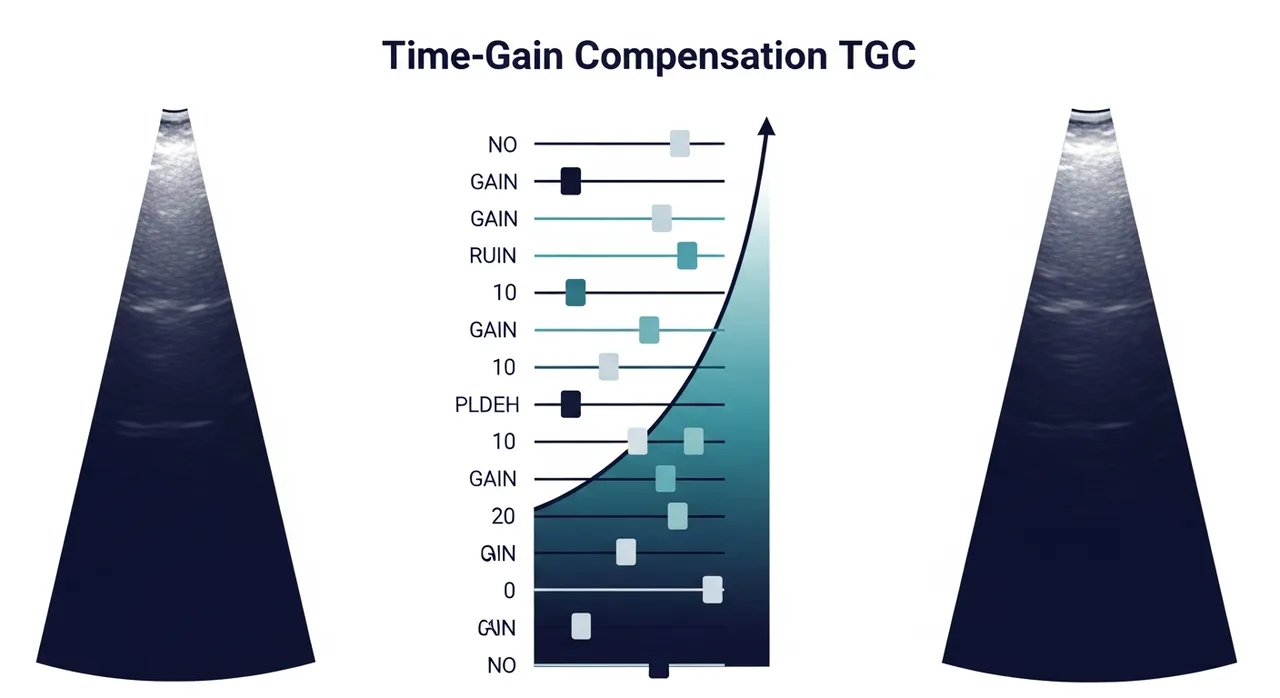
What it does: Applies depth-dependent gain to compensate for the progressive attenuation of returning echoes from deeper tissue.
Physics: Returning echoes from deep structures have traveled farther and lost more amplitude to attenuation. TGC adds extra gain to the late-arriving echoes so that an evenly echogenic medium (like a uniform liver) appears uniformly bright top to bottom.
Set TGC correctly by scanning a uniform region, then adjusting the slider stack so the brightness is even from skin line to deepest field. The classic shape is a gentle upward curve — minimal gain at the top, more gain in the middle, even more at the bottom.
Common errors: Banding (one slider clearly out of line, producing a bright or dark horizontal band), over-compensation in the near field that washes out subcutaneous detail, and under-compensation in the far field that makes deep structures look hypoechoic when they are actually normal.
Trade-off: TGC is corrective rather than tradeoff-laden, but a sloppy curve will hide pathology by either over-brightening normal tissue or shadowing real lesions.
SPI relevance: Expect images with obvious banding artifacts and a question asking which slider to move.
Depth
What it does: Sets the maximum imaging depth displayed on the screen.
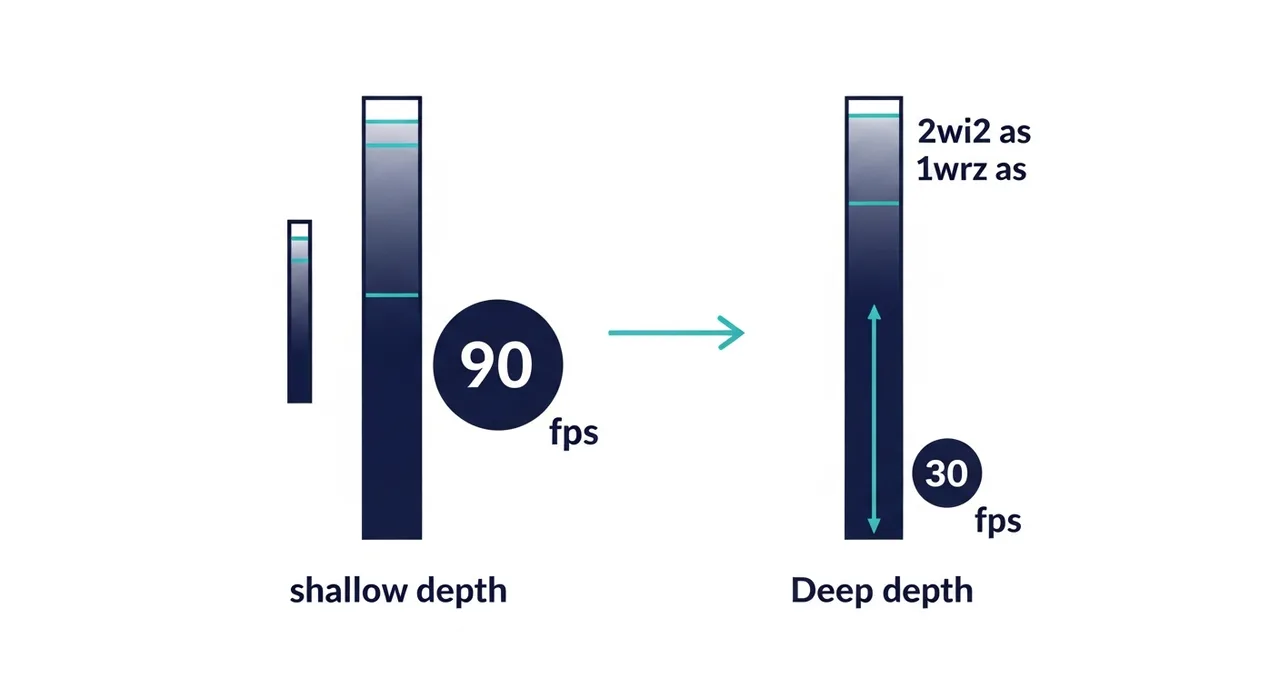
Physics: The machine must wait for the deepest echo of one pulse to return before sending the next. Doubling depth roughly halves the maximum possible pulse repetition frequency (PRF) and therefore frame rate.
Increase depth when the structure of interest extends beyond the current field, or you need to evaluate posterior anatomy and shadowing.
Decrease depth when the structure of interest occupies less than the lower third of the screen. Filling the screen with the structure of interest improves perceived resolution and frees frame rate for other uses.
Trade-off: Deeper imaging costs frame rate and slows color/Doppler responsiveness. Shallower imaging frees frame rate and lets you use more focal zones, more line density, or wider color boxes without temporal penalty.
SPI relevance: PRF–depth–frame-rate relationships are heavily tested. Know the chain: greater depth → lower max PRF → lower frame rate → lower temporal resolution.
Focus and Focal Zones
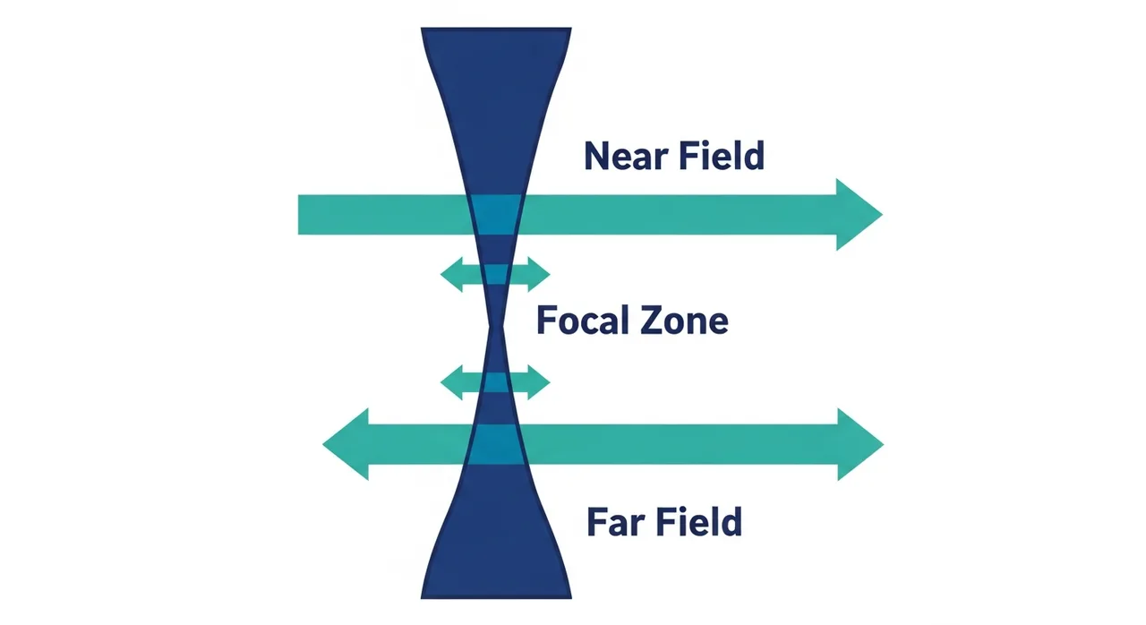
What it does: Narrows the beam at a chosen depth (or depths), improving lateral resolution there.
Physics: Electronic focusing delays signals to and from individual elements so that the beam waist sits at a chosen depth. Lateral resolution is best at the focal zone and degrades above and below it.
Place the focal marker at or just below the structure of interest. For most B-mode work, one focal zone parked at the lesion is correct.
Use multiple focal zones when you need uniform lateral resolution across a deep field, accepting the frame-rate penalty.
Trade-off: Each additional focal zone is a separate transmit event. Two focal zones roughly halve frame rate; four roughly quarter it. In cardiac and fetal cardiac imaging the temporal cost is usually unacceptable, so single focal zone with thoughtful placement is the norm.
SPI relevance: Lateral resolution and beam width are core SPI topics. Expect questions on why frame rate falls when focal zones are added.
Dynamic Range and Compression
What it does: Maps the range of returning echo amplitudes onto the displayable grayscale.
Physics: Real echo amplitudes span a huge dynamic range — often 80 to 120 dB — but the display only shows perhaps 256 levels of gray. Dynamic range (sometimes labeled compression) is the curve that maps real amplitudes onto displayed grays.
Increase (wider) dynamic range when you want a softer, more gradient-rich image with subtle tissue differentiation. Useful in obstetrics, abdominal parenchymal imaging, and breast.
Decrease (narrower) dynamic range when you want a high-contrast image with harder edges. Useful in cardiac wall motion analysis and in border definition for measurements.
Trade-off: Wide dynamic range buries pathology behind soft transitions. Narrow dynamic range can hide subtle lesions in a uniform background by over-flattening the gradient.
SPI relevance: Dynamic range and the log compression curve appear in most SPI banks; know that it is a post-processing display function, not a transmit setting.
Sector Width
What it does: Narrows or widens the lateral extent of the image.
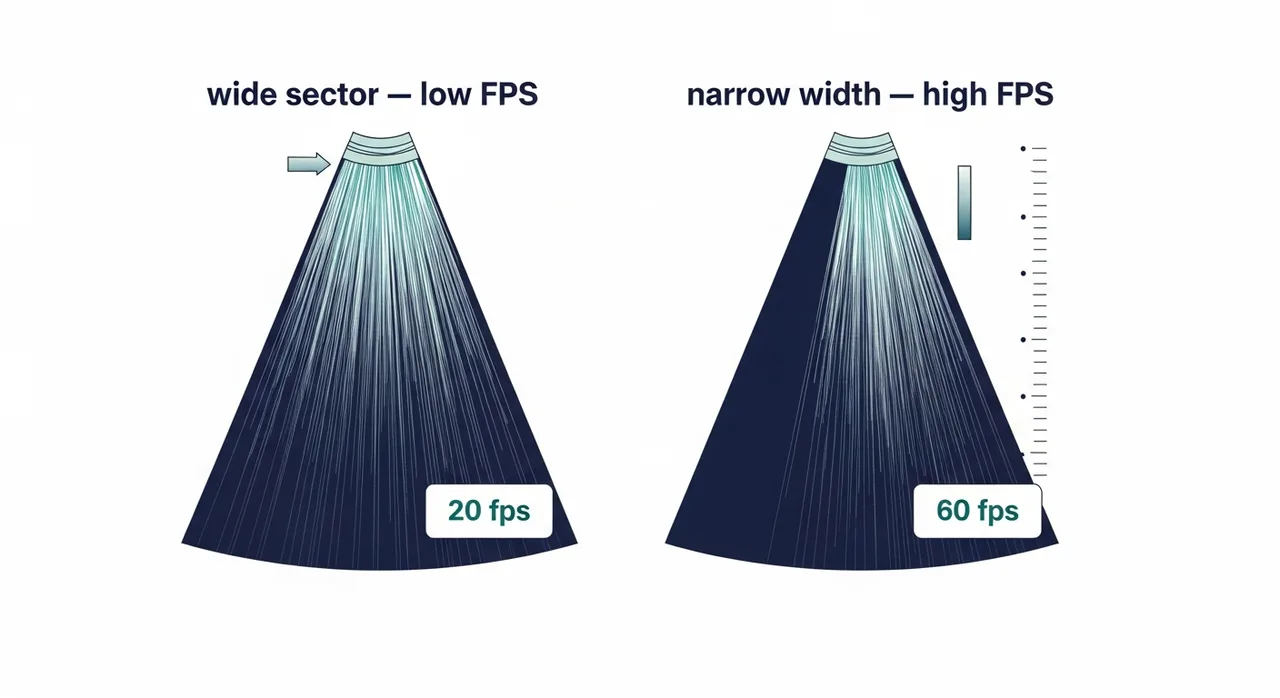
Physics: Frame rate is inversely proportional to the number of scan lines per frame. A narrower sector contains fewer lines, so each frame is built faster.
Narrow the sector when you need higher frame rate — fetal cardiac, color Doppler over a focal vessel, any application where motion temporal resolution matters more than panoramic view.
Widen the sector when you need anatomic context, such as during an initial survey scan or when measuring across a wide structure.
Trade-off: Field of view versus frame rate.
Line Density
What it does: Controls the number of scan lines per degree of sector width.
Physics: More lines per sector improves lateral sampling and therefore lateral resolution, at the cost of frame rate.
Increase line density when you need fine lateral detail in a static or slow-moving structure — superficial mass characterization, slow venous flow.
Decrease line density when temporal resolution dominates — cardiac, fetal heart, rapid Doppler interrogation.
Trade-off: Lateral resolution versus frame rate. This is the same trade as focal zones from a different angle.
Persistence (Frame Averaging)
What it does: Blends each new frame with previous frames to smooth the displayed image.
Physics: Persistence is a temporal low-pass filter. It reduces speckle and electronic noise by averaging across frames, but it also smears moving structures.
Increase persistence when the image is noisy and the structure is essentially static — abdominal parenchymal imaging, slow venous flow, characterizing a mass.
Decrease persistence when anything is moving fast — cardiac walls, valves, fetal heart, rapid Doppler color. Excess persistence in cardiac imaging produces ghosting and false thickening of the myocardium during systole.
Trade-off: Image smoothness versus temporal accuracy. The classic example: a beautiful smooth carotid wall on persistence 4 looks great until you realize the systolic-diastolic motion has been averaged into a blur.
Tissue Harmonic Imaging (THI)
What it does: Transmits at a fundamental frequency and listens at the second harmonic (twice the transmit frequency) generated within tissue.
Physics: Harmonic generation increases with depth and is greatest along the central beam axis. Side-lobe and reverberation artifacts, which arise from lower-amplitude off-axis energy, generate weaker harmonics. Imaging at the harmonic therefore filters out much of that artifact noise and improves contrast resolution.
Use THI when the patient is technically difficult — high BMI, poor cystic-versus-solid differentiation, near-field clutter in a fluid-filled structure, suboptimal cardiac windows.
Turn THI off when you need maximum penetration on an already attenuating patient. Because you are listening at twice the transmit frequency, harmonic penetration is somewhat less than fundamental at the same nominal probe frequency.
Trade-off: Cleaner image and better contrast resolution at the cost of slightly reduced penetration and somewhat lower temporal resolution on some platforms.
SPI relevance: Expect questions distinguishing fundamental from harmonic imaging and asking why harmonics reduce side-lobe artifact.
Spatial and Frequency Compounding
What it does: Combines multiple lines of sight (spatial compounding) or multiple transmit frequencies (frequency compounding) into a single displayed frame.
Physics: Speckle and many artifacts are angle- or frequency-dependent. Looking from several angles or at several frequencies and averaging the results suppresses those angle/frequency-dependent features while reinforcing real reflectors.
Use compounding when speckle is interfering with lesion detection, or when you want to soften acoustic shadows behind ribs or bowel gas.
Turn compounding down or off when you actually want shadows and edge enhancements as diagnostic clues — gallstones, calcifications, posterior acoustic enhancement behind cysts. Compounding can soften these classic findings into ambiguity.
Trade-off: Reduced speckle and artifact at the cost of softened real edges and lower frame rate.
Color and Power Doppler Controls
Color Gain
What it does: Amplifies the color-coded Doppler signal within the color box.
Set it by turning color gain up until color noise just begins to appear in stationary tissue, then backing off slightly. Below that level you lose real low-amplitude flow; above it you fill the box with random noise.
Trade-off: Sensitivity to slow flow versus background noise.
Color Box Size and Position
What it does: Defines the region of interest where color Doppler is applied.
Physics: Inside the color box, the machine fires multiple pulses per scan line to estimate Doppler frequency shift. Larger boxes mean more lines and more pulses per frame, which lowers frame rate.
Keep the color box as small as possible — just large enough to cover the vessel or area of interest, and steered to maintain a favorable Doppler angle.
Trade-off: Coverage versus frame rate. A wide color box across an entire abdomen is cinematically impressive and clinically useless if it drops frame rate to 6 Hz.
Color PRF / Scale
What it does: Sets the pulse repetition frequency for the color Doppler interrogation, which determines the velocity range displayed without aliasing.
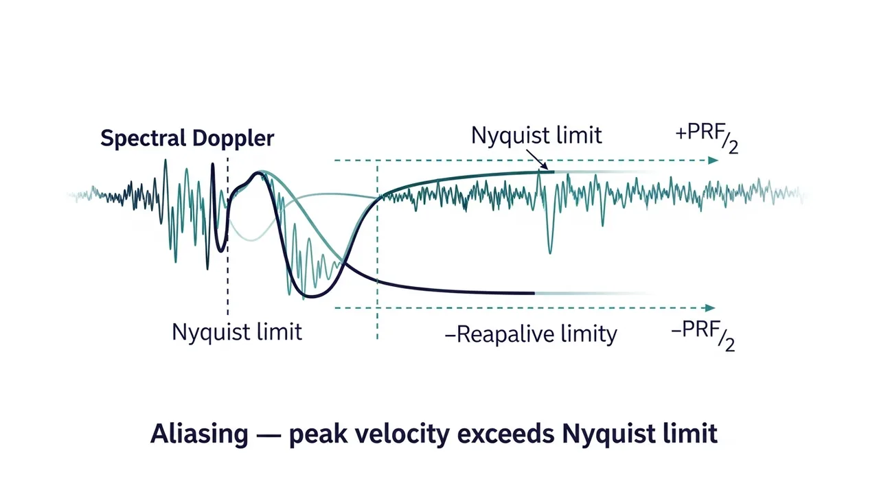
Physics: Aliasing occurs when the actual Doppler shift exceeds half the PRF (the Nyquist limit). Higher PRF raises the Nyquist limit and resolves higher velocities, but it also reduces sensitivity to slow flow.
Increase PRF when flow is high and the color box is full of aliasing (color wrapping or mosaic).
Decrease PRF when you need to detect slow flow — venous, low-velocity arterial, post-stenotic recovery.
Trade-off: High velocity range versus slow-flow sensitivity. You cannot tune both at once on the same color box.
SPI relevance: Nyquist, aliasing, and PRF–depth interactions are heavily tested. Remember the chain: deeper sample → lower max PRF → easier to alias high-velocity flow.
Wall Filter
What it does: Removes low-frequency Doppler signals that arise from vessel-wall and tissue motion.
Physics: Vessel walls move slowly compared with blood. A high-pass filter rejects signals below a chosen frequency cutoff.
Increase wall filter when wall motion artifact is contaminating the signal in a high-flow vessel.
Decrease wall filter when you are looking for slow venous or low-velocity arterial flow that would otherwise be filtered out as if it were wall motion.
Trade-off: Clean trace versus loss of slow real flow. The classic miss is a low-velocity flow in a near-occluded carotid bulb hidden behind an aggressively high wall filter.
Color Persistence
What it does: Frame averaging applied to the color overlay.
Trade-off: Smooth color appearance versus accurate timing of flow events. In valvular regurgitation or fetal cardiac flow assessment, excessive color persistence prolongs the apparent duration of jets.
Baseline Shift
What it does: Moves the zero-velocity baseline up or down within the color or spectral display.
Use it when flow is unidirectional and you are wasting half the available velocity range on a direction that will never carry signal. Shifting the baseline doubles the effective Nyquist limit in the direction of actual flow.
Trade-off: None when used correctly — this is one of the few free wins on the panel.
Steering Angle
What it does: Electronically angles the color or Doppler beam relative to the linear array face.
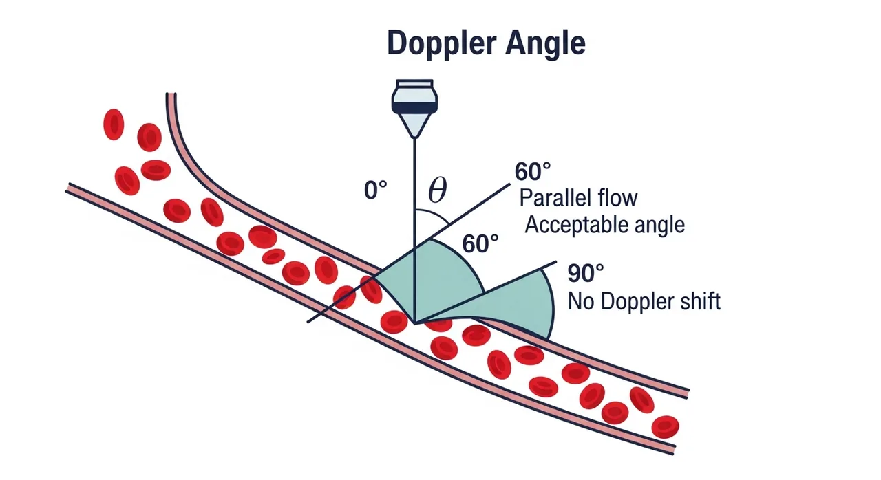
Physics: The Doppler equation depends on the cosine of the angle between the beam and the direction of flow. At 90 degrees the cosine is zero and Doppler shift vanishes. The goal is to keep the insonation angle at or below 60 degrees for accurate velocity quantification.
Steer the color box so that the apparent flow direction in the vessel runs at a favorable angle, not perpendicular to the beam.
Trade-off: Steering does cost some lateral resolution at the steered edge of the image, but the diagnostic gain in Doppler accuracy is almost always worth it.
Spectral (Pulsed-Wave) Doppler Controls
Sample Volume Size and Position
What it does: Defines the depth and length of the gate from which spectral Doppler signal is sampled.
Set it by placing the gate inside the vessel, centered in the lumen, sized to roughly two-thirds of the vessel diameter for normal velocity sampling. For peak velocity at a stenosis, use a smaller gate placed precisely at the highest-velocity point identified by color.
Trade-off: A larger gate captures more flow profile and is more forgiving but introduces spectral broadening. A smaller gate is more precise but easier to misplace.
Spectral PRF and Aliasing
Same physics as color PRF. Increase PRF to resolve high velocities (post-stenotic jets, AV fistulas), decrease PRF to capture slow flow. Spectral aliasing produces wrap-around at the top or bottom of the velocity scale.
Wall Filter (Spectral)
Same logic as color wall filter. Keep low when hunting for slow or near-occlusive flow; raise when wall thump is contaminating the trace.
Angle Correction
What it does: Tells the machine the assumed angle between the beam and the direction of flow so it can convert measured Doppler shift into a velocity in cm/s.
Critical rule: Angle correction is only as accurate as the operator's alignment of the cursor with true flow. The cursor must lie along the long axis of the vessel and the angle should be 60 degrees or less. Above 60 degrees, small angle errors produce large velocity errors because the cosine curve steepens rapidly.
SPI relevance: Expect direct calculations using the Doppler equation and questions on angle-related velocity errors.
Sweep Speed
What it does: Controls how quickly the spectral trace scrolls across the display.
Increase sweep speed when you want to evaluate beat-to-beat morphology, such as systolic upstroke time or spectral broadening details.
Decrease sweep speed when you want to see more cardiac cycles at once, such as during a respiratory variation evaluation.
Continuous-Wave Doppler
What it does: Uses two separate elements — one continuously transmitting, one continuously receiving — to measure very high velocities without aliasing.
Physics: Because there is no pulsing, there is no PRF and therefore no Nyquist limit. The trade is that range resolution is lost — you measure all velocities along the entire beam path, not from a specific depth gate.
Switch to CW when the velocity exceeds what PW can resolve even with PRF and baseline maxed out. Classic uses: aortic stenosis peak velocity, tricuspid regurgitation jet for pulmonary pressure estimation, dialysis fistula flow.
Trade-off: No depth resolution. You cannot tell where along the beam the velocity arose, so anatomic placement of the cursor is critical.
SPI relevance: PW versus CW comparisons are standard exam material. Know which gives depth resolution and which avoids aliasing.
Power Output, MI, and TI — The ALARA Controls
What they do: Power output controls the acoustic energy transmitted into the patient. Mechanical Index (MI) and Thermal Index (TI) are real-time displayed estimates of the potential bioeffects of that energy.
Physics: MI estimates the likelihood of cavitation in tissue containing gas (lung, bowel, contrast agents). TI estimates tissue heating and is reported as TIS (soft tissue), TIB (bone, important in obstetrics past the first trimester), or TIC (cranial).
ALARA principle (As Low As Reasonably Achievable): Use the lowest output and shortest dwell time consistent with obtaining diagnostic information. Increase power only after you have optimized gain, depth, focus, and frequency. In obstetric imaging, especially first trimester and during prolonged Doppler, keep MI and TI low and dwell time short.
Trade-off: Sensitivity and depth penetration versus patient exposure.
SPI relevance: ALARA, MI/TI definitions, and the higher patient exposure of pulsed Doppler relative to B-mode are exam staples.
Zoom — Read Zoom vs. Write Zoom
Read zoom (display zoom) simply enlarges a portion of the already-acquired image by interpolation. The displayed pixels get bigger; no new acoustic information is gathered. It is fast and convenient but it does not improve resolution.
Write zoom (RES or HD zoom) restricts the active acoustic field to a smaller region and re-acquires it with the full available line density and frame rate dedicated to that smaller area. Real lateral resolution improves. Frame rate often improves as well, because the machine no longer wastes lines outside the zoomed area.
Use write zoom when you are about to take measurements or characterize a small lesion. Read zoom is fine for showing a finding to a colleague at the workstation.
SPI relevance: Distinguishing read zoom from write zoom — and understanding which one actually improves resolution — is a classic exam item.
Cine and Clip Capture
Cine review lets you scroll back through the most recent buffered frames to capture the precise moment that best demonstrates a finding. Practical workflow: keep persistence low when you need clean cine for valve motion or fetal cardiac, set clip duration to capture full cardiac or respiratory cycles when relevant, and label your stored clips with anatomy and projection so the interpreting physician does not have to guess.
How These Controls Interact
The single most important concept in knobology is that the controls are coupled. Turn one knob and others move whether you wanted them to or not. A few of the most consequential interactions:
Depth → frame rate → persistence. Increasing depth lowers the maximum PRF and therefore frame rate. If you then forget to lower persistence, the cardiac structures you went deeper to see will smear in motion. This is why depth changes in cardiac imaging often require a follow-up persistence adjustment.
Focal zones → frame rate. Each added focal zone is another transmit event. Two zones halve frame rate. Use multiple zones in static abdominal work; commit to a single well-placed zone in cardiac and fetal cardiac.
Color box size → frame rate → temporal accuracy of flow events. A color box that covers the whole abdomen drops frame rate so far that you can no longer distinguish systolic from diastolic flow. Keep the box just large enough.
PRF → aliasing and slow-flow sensitivity. High PRF resolves high velocities and ignores slow flow. Low PRF picks up slow flow and aliases on jets. There is no setting that does both.
Frequency → resolution and penetration. Going to a higher-frequency probe to chase axial resolution will fail if the structure is below the new probe's penetration. Choose the lowest frequency that still resolves the structure adequately.
THI → penetration and frame rate. Harmonic imaging cleans up the image but costs you a little depth and, on some platforms, a little frame rate. On the most difficult patients, fundamental imaging at low frequency may still beat THI at depth.
Image-Optimization Recipes by Scenario
Deep Abdomen on a Large Patient
Lower-frequency curved array (2–3 MHz). Set depth to fit the structure of interest in the lower two-thirds of the screen. Single focal zone parked at the lesion. Tissue harmonic imaging on. Increase persistence modestly (the structures are largely static). TGC curve evenly distributed top to bottom. Increase output power last, only after optimizing the rest, respecting ALARA.
Fetal Heart
Curved array around 4–6 MHz, or an appropriate phased array if available. Narrow sector centered on the fetal chest. Single focal zone at the heart. Persistence low to capture valve motion crisply. Frame rate goal of 60 Hz or higher; if you cannot reach it, reduce sector, line density, or depth before increasing power. Color box small, color PRF appropriate to expected fetal cardiac velocities, color persistence low. Keep MI/TI low and dwell time short.
Carotid Doppler
Linear array around 7–10 MHz. Steer the color box and PW cursor for an angle of 60 degrees or less. Color PRF set to the expected peak systolic velocity range, then adjusted up if aliasing or down if slow flow is suspected. Wall filter low enough to detect slow near-occlusive flow but not so low that wall thump dominates. Sample volume positioned in the center of the lumen, sized to roughly two-thirds of the vessel. Angle correction cursor aligned with true flow direction.
Superficial MSK
High-frequency linear probe (12–18 MHz or higher). Shallow depth. Single focal zone at the structure (or use write zoom). Tissue harmonic imaging often improves contrast in tendon-fluid interfaces. Compounding off when you want to preserve characteristic tendon fibrillar pattern and bony shadowing.
Pediatric Echo
Higher-frequency phased array than adult. Narrow sector. Single focal zone. Persistence at minimum. Maximize frame rate aggressively — pediatric cardiac structures move fast and are small, so both temporal and spatial resolution must be high. Color box minimal, PRF tuned to expected velocity range.
Slow Venous Flow
Lower color and spectral PRF than the default preset. Lower wall filter. Increase color gain just below the noise threshold. Compounding can help fill in low-amplitude signal. Patient maneuvers (augmentation, Valsalva) often produce more diagnostic information than any knob change.
Knobology and the SPI Exam
The SPI exam tests whether you understand the physics behind the controls — not whether you have memorized a vendor's button names. Expect items that ask you to predict what happens to frame rate when you change depth or sector width, to identify the trade-off behind a specific image artifact, to apply the Doppler equation, to distinguish receive gain from transmit power, to choose between PW and CW, and to apply ALARA in obstetric Doppler scenarios. Our companion guide on the core SPI physics concepts walks through the underlying physics in detail, and the complete ARDMS SPI exam guide covers the full exam structure and study plan. For a study approach that pairs naturally with knobology drilling, see AI-powered study tools for ARDMS exam prep.
Frequently Asked Questions
Q: What is the single highest-yield knob to learn first?
TGC. A correctly set TGC curve fixes more diagnostic ambiguity than almost any other single adjustment, and an incorrectly set TGC will hide pathology no matter how perfectly you have tuned everything else.
Q: When should I move off the preset entirely?
Anytime the image you have is not answering the clinical question. Presets are starting points, not contracts. The instant you find yourself accepting a marginal image because the preset said this is what an OB second trimester scan should look like, optimize off-preset.
Q: How do I prevent over-gain from masking real pathology?
After you set gain, look at a known anechoic structure in the field — gallbladder, vessel lumen, fluid-filled bladder. It should appear black with no internal echoes. If it is filled with low-level gray noise, you are over-gained. This habit takes ten seconds and prevents an entire class of false positives.
Q: Why does my color Doppler look mosaic and chaotic in a clearly patent vessel?
Almost always aliasing from a too-low color PRF for the velocity actually present, or insonation at too steep an angle producing inconsistent direction encoding. Raise PRF first; if that does not resolve it, check your steering angle.
Q: Do I need to understand the physics if I will only ever scan clinically?
Yes. Producing diagnostic images on hard patients depends on understanding why each control behaves the way it does. The boards test the physics because the physics is what makes you a competent operator at the bedside.
Q: How does knobology differ between B-mode and Doppler optimization?
B-mode optimization is mostly about resolution-versus-penetration trades and TGC. Doppler optimization adds the angle, PRF/Nyquist, and wall filter trades on top of B-mode. The discipline is the same — name the trade, then make it deliberately — but Doppler is less forgiving of careless settings because both false-positive flow (over-gain) and false-negative flow (over-filtering) carry diagnostic consequences.
Q: Where should a working sonographer adding a registration focus first?
If you are already comfortable with B-mode optimization in your current specialty, the highest-yield areas are typically Doppler physics, ALARA in obstetric scenarios, and the depth–PRF–frame-rate chain. Pair this guide with our SPI practice questions and the relevant clinical specialty bank for your new credential.
Conclusion: Trade Deliberately, Not by Accident
Every image you produce is the result of a stack of trade-offs the machine makes for you when you accept a preset, and that you make for yourself the moment you start turning knobs. Understanding those trades helps you produce diagnostic images on patients who would otherwise be called technically limited, and answer SPI questions from understanding rather than from memorized facts. When you are ready to drill the physics in a structured way, start with our SPI practice questions, then move into your specialty practice banks. The knobs in front of you are a physics interface — once you learn to speak the language, the patient and the pathology will tell you which trade to make.
Sources
- AIUM Practice Parameters and Technical Standards — American Institute of Ultrasound in Medicine
- ALARA Principle in Diagnostic Ultrasound — AIUM
- ARDMS SPI Examination Content Outline — ARDMS
- Doppler Ultrasound Physics — RadiologyKey Reference — Radiology Key
If you find this article helpful and want to put the strategies into practice, sign up for an Ultrasound Analytics account to access the full ARDMS-aligned question bank, AI tutoring on every missed answer, full-length timed exams, and the analytics dashboard that translates your performance into a Readiness Score for each specialty registration.